The Quick Answer
Getting C-mount FA lens selection right boils down to three sentences. First, the lens image circle must fully cover your sensor diagonal. Second, its optical resolution must meet or exceed your sensor’s Nyquist frequency. Third, your working distance and field of view determine the focal length — everything else is secondary. Only after these three are settled should you trade off aperture, distortion limits, mechanical constraints and focus control. The seven steps below turn that logic into a repeatable checklist.
Step 1: Start from the Sensor — Image Circle and lp/mm Matching
Most selection errors start here, so start here. If you are still deciding which type of lens the task needs, our machine vision optics guide covers the four variables and the physical limits first.
Image circle ≥ sensor diagonal. A lens projects a circular image; the usable diameter of that circle is the image circle. If the image circle is smaller than your sensor diagonal, the corners will be dark and out of focus — no software correction can recover information that never reached the sensor.
A 2/3″ sensor has an ~11 mm diagonal and needs a lens with an 11 mm or larger image circle.
A 1.1″ sensor is nominally 17.6 mm on the diagonal — and the 24.5 MP parts actually shipping in that class run to roughly 19 mm. A “2/3″-format” lens, however sharp on axis, will vignette badly on a 1.1″ sensor.
Optical resolution ≥ sensor Nyquist frequency. A sensor can only exploit detail up to its Nyquist limit:
Nyquist (lp/mm) = 1 / (2 × pixel pitch in mm)
Example A — 2.74 µm pixels, the pitch behind today’s 1.1″-class 24.5 MP sensors: Nyquist ≈ 1 / (2 × 0.00274) ≈ 182 lp/mm. The lens must deliver meaningful MTF at 182 lp/mm not only in the center but toward the corners of a ~19 mm circle. A generic “5 MP” lens cannot.
Example B — 2/3″ 10 MP sensor, 2.5 µm pixels: Nyquist ≈ 200 lp/mm on an 11 mm circle. This is even more demanding per millimeter, which is why Josight publishes MTF curves at the Nyquist frequency for every model instead of simply sticking a “megapixel” label on it.
Rule of thumb: check the lens datasheet’s image circle and MTF-at-Nyquist first — and treat marketing “megapixel” ratings with skepticism.
Step 2: Fix the Focal Length from Working Distance
Once sensor coverage is confirmed, geometry gives you the focal length:
FOV ≈ Sensor width × WD / f → f ≈ Sensor width × WD / FOV
This is the thin-lens approximation, and it is accurate enough while the magnification m = sensor width / FOV stays small. The exact relation is f = m·WD/(1+m): at m = 0.03 the approximation is within 3%, but at m = 0.2 it underestimates by 20%, and at m = 0.5 by 33%. Anywhere near macro or high-magnification gauging, use the exact form.
Worked example: a 2/3″ sensor (9.6 mm wide), working distance 250 mm, required field of view 300 mm:
f ≈ 9.6 × 250 / 300 ≈ 8 mm → choose an 8 mm FA lens.
Two practical notes:
Compute WD from the front of the lens barrel, and include any protective window or filter thickness.
Leave a 10–20% WD margin. If your product positions vary by ±20 mm, a lens whose nominal WD sits exactly at the tolerance edge will drift out of focus.
Josight’s 8 / 16 / 25 / 35 / 50 mm series covers the common FOV–WD combinations for 2/3″ and 1.1″ sensors; pick the focal length whose nominal WD centers your tolerance band, not the one that merely reaches it.
Step 3: Aperture — Depth of Field Versus Light Versus Diffraction
Aperture is a three-way trade-off:
Open (low F-number): more light, shorter exposure, but shallow depth of field and residual aberrations.
Closed (high F-number): more depth of field, but diffraction softens detail. At f/8 the Airy disk measures ≈ 2.44 × 0.55 µm × 8 ≈ 10.7 µm — about four 2.5 µm pixels across. But the decisive test is not that ratio; it is the diffraction cut-off 1/(λN) against sensor Nyquist 1/(2p). At f/8 the cut-off is 227 lp/mm, while a 2.5 µm sensor needs 200 lp/mm — so f/8 is still usable. Two stops further, at f/11, the cut-off falls to 165 lp/mm and you are genuinely discarding pixels. On a 2 µm sensor (Nyquist 250 lp/mm) the wall arrives earlier: f/8 already fails and the window closes near f/5.6.
For most FA lenses on 2.5–3.45 µm pixels, the optical sweet spot is f/4 – f/5.6: aberrations are well corrected, diffraction remains acceptable, and there is sufficient light. On ≤2.5 µm pixels the window shifts toward the open end and f/2.8 becomes usable — not because diffraction got better, but because you can no longer afford to stop down.
If your application has flat, single-plane targets (code reading, surface OCR), work near the sweet spot. If you need depth (parts sitting at different heights), choose the smallest F-number that still keeps your tolerance band in focus, then add light or gain as needed.
A physical limit worth knowing: the diffraction–pixel tension gets worse as pixels shrink. On 2.x µm sensors the usable window narrows to roughly f/2.8–f/5.6, with f/4 usually the best compromise between residual aberration and diffraction, because stopping down to gain DOF spends pixel resolution first. There is no F-number that maximizes light, DOF and sharpness simultaneously — the laws of optics, not the price tier, set that boundary.
Step 4: Distortion Limits — Set Them by Application
Distortion bends straight lines; how much you can tolerate depends on what the vision system does:
Application | Recommended distortion limit |
|---|---|
Precision measurement / gauging | ≤ 0.1% (plus software calibration) |
Defect inspection, presence checks | ≤ 0.3–0.5% |
Code reading, OCR, guidance | ≤ 1% |
Distortion is worse at the field edges, so evaluate it across the full FOV, not just the center. For measurement tasks, prefer low-distortion designs and budget for a one-time calibration with a grid target even when the lens is rated ≤ 0.1%.
Know what software can and cannot fix. Correctable: radial and tangential distortion at a fixed WD with a stable calibration; lateral chromatic aberration (per-channel resampling); vignetting and illumination falloff (flat-field); fixed-pattern noise; and mild defocus, if the PSF is known and SNR is high (real gains are typically 1.5–2×, not a miracle). Not correctable: anything beyond the diffraction cut-off 1/(λN), anything outside the image circle (literally zero signal), aliasing and moiré, saturated or clipped highlights, and depth information absent from a single view. Calibration complements good optics; it does not replace them.
Step 5: Mechanical Parameters — Length, Filter Thread, Locks
The optics pass review — then the station integrator calls. Check:
Overall length and diameter: a 50 mm FA lens can exceed 70 mm in barrel length; verify clearance against lighting, enclosures and robot paths.
Filter thread: if you plan to use polarizers, protective windows, or band-pass filters, confirm the thread size (e.g., M27 × 0.75) exists on the focal length you chose — not just on the popular models.
Focus and iris locks: vibration-heavy environments (packaging lines, CNC cells) need set screws to prevent focus and aperture drift.
Step 6: Motorized or Manual Focus?
For a fixed station inspecting one product at one height, a manual-focus lens with locking screws is a set-and-forget solution — the most economical choice.
Motorized (electric-focus) versions earn their premium when working distance changes between products or batches, when stations are hard to reach or deployed remotely, or when many cameras must be reconfigured by recipe. The optics are typically the same; you are paying for a closed-loop drive and repeatability. At Josight the motorized and manual versions share the identical optical platform, so a field upgrade needs no new optical design and typically only a single-scale recalibration. See our companion article, “Motorized vs Manual FA Lenses: When Does Electric Focus Actually Pay Off,” for the full decision logic.
Step 7: Batch Consistency and Test Data
If you are deploying a single camera, one excellent lens is all you need. If you build machines — ten, a hundred, or a fleet that your customers reconfigure in the field — you need consistency:
Per-lens, serialized MTF and distortion test reports, not just type curves.
Tight focus-position tolerance across a batch so a lens can be swapped without refocusing the station.
Documented manufacturing revisions so a replacement lens behaves like the one it replaces.
Ask the supplier for sample test reports before finalizing a design-in. A datasheet tells you what one prototype achieved; a test report tells you what you will actually receive. Josight ships FA lenses with per-unit measured data precisely because the difference between a type curve and a serialized report is exactly the gap that shows up on your production line.
Three Common Selection Mistakes
Buying a “high-megapixel” lens for a high-resolution sensor. The “megapixel” label is marketing — only the MTF-at-Nyquist curve over your sensor’s image circle matters.
Ignoring image circle until corners go dark. A 2/3″-format lens on a 1.1″ sensor is not “slightly cropped” — it is unusable.
Leaving no working-distance margin. Nominal WD that sits exactly at the product tolerance edge will produce intermittent defocus that no one can reproduce on the bench.
Forward View: Where C-Mount Selection Is Heading
Three shifts will change how this checklist is applied over the next few years:
• 50 MP-class sensors and 2.x µm pixels move mainstream. The limiting factor is migrating from the camera to the lens: corner MTF, decenter and stray light decide how many of those pixels are truly usable. Expect Nyquist-referenced, field-resolved MTF to become a minimum expectation rather than a differentiator.
• AI-assisted lens selection. Configurators that ingest sensor datasheet, WD and feature size and shortlist candidates automatically are already appearing. They are only trustworthy when trained on measured per-lens data — which is why measured, not nominal, curves remain the real moat.
• The C-mount ceiling — and why it is mechanical, not optical. Two hard numbers set it. First, the 17.526 mm flange distance leaves only a few millimetres behind the mount for the rear group, which is why short focal lengths run out of room as the format grows. Second, the 1″-32 thread is 25.4 mm across with roughly 22–23 mm of clear aperture, so the usable image circle is capped around 22–24 mm — which is exactly why 4/3″ (21.6 mm) is the practical limit. The real format ladder above C-mount runs 1.1″ (17.6 mm) → 4/3″ (21.6 mm) → APS-C (28.1 mm) → APS-H / full frame (43.3 mm), with large-format industrial sensors such as 1.8″ (e.g. 127 MP at 3.45 µm) requiring F-mount, M42×1, M48, M58×0.75, M72×0.75 or M90. Design your mechanics so a mount change is not a full redesign when your next camera generation arrives.
FAQ
Q1: Can I use a 2/3″ lens on a 1.1″ sensor?
No. The 11 mm image circle cannot cover the 17.6 mm diagonal, and the corners will be black. The only exception is a deliberate center-ROI application — in which case re-evaluate MTF over that ROI, because the lens was never optimized for it either.
Q2: How do I know how many lp/mm my lens needs?
Take your pixel pitch in millimeters and compute 1 / (2 × pitch). A 2.74 µm sensor needs ~182 lp/mm; a 3.45 µm sensor needs ~145 lp/mm.
Q3: Does a “25 MP lens” make my 2/3″ 10 MP camera sharper?
Only if its MTF at your sensor’s Nyquist frequency (200 lp/mm for 2.5 µm pixels) is higher than your current lens at the same frequencies, across the field. Compare curves, not labels.
Q4: C-mount or S-mount?
C-mount has a 17.526 mm flange distance and suits larger sensors (2/3″ and above) with robust industrial barrels. S-mount (M12) has a ~12.5 mm flange and suits compact 1/2″-and-below sensors. For factory automation at 5 MP and above, C-mount FA lenses are the standard choice.
Q5: Can’t software just correct distortion and soft corners?
Stable distortion at fixed WD — yes, with calibration. Softness from low MTF, diffraction, defocus and image-circle vignetting — no; that information was never captured. Parallax from part height requires a telecentric lens, not a software setting.
Q6: How far can I push a C-mount lens on sensor format?
Around 1.1″ is today’s practical sweet spot across the full focal-length range; 4/3″ (21.6 mm) is the hard ceiling for C-mount. Larger formats are possible at longer focal lengths, but short-focal-length lenses beyond ~1.1″ run into flange-distance geometry and generally move to F-mount or larger mounts. Always check corner MTF on your exact sensor.
Get a Shortlist in 24 Hours
Send your sensor specifications and working distance to Josight — we will shortlist three C-mount FA lens models for you, complete with MTF curves at your Nyquist frequency and distortion charts, within 24 hours.
Disclaimer
The information provided in this blog post is for general informational purposes only. Lens specifications, performance data, and product availability are subject to change without notice. Actual performance may vary depending on application conditions, system configuration, and environmental factors. Josight makes no warranties, express or implied, regarding the accuracy, completeness, or suitability of the information contained herein. Readers should conduct their own testing and validation before making procurement decisions.